To multiply a matrix by a single number is easy:
- These are the calculations: 2×4=8. 2×0=0.
- The "Dot Product" is where we multiply matching members, then sum up: (1, 2, 3) • (7, 9, 11) = 1×7 + 2×9 + 3×11. = 58.
- (1, 2, 3) • (8, 10, 12) = 1×8 + 2×10 + 3×12. = 64.
- DONE! Why Do It This Way?
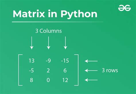
Matrix is a way of arrangement of numbers, sometimes expressions and symbols, in rows and columns. Matrix formulas are used to solve linear equations and calculus, optics, quantum mechanics and other mathematical functions.
Calculating the exponential value in Python
- base = 3. exponent = 4. print "Exponential Value is: ", base ** exponent. Run.
- pow(base, exponent)
- base = 3. exponent = 4. print "Exponential Value is: ", pow(base, exponent) Run.
- math. exp(exponent)
- import math. exponent = 4. print "Exponential Value is: ", math. exp(exponent)
solve(expression) method, we can solve the mathematical equations easily and it will return the roots of the equation that is provided as parameter using sympy. solve() method. Syntax : sympy.solve(expression) Return : Return the roots of the equation.
Method 1
- Convert the system of equations to matrix form:
- Import the numpy module and write the matrices as numpy arrays.
- Define coefficient and results matrices as numpy arrays A = np.array([[5,3],[1,2]]) B = np.array([40,18])
- Use numpy's linear algebra solve function to solve the system C = np.linalg.solve(A,B)
The standard formula of a quadratic equation in Python is ax^2+bx+c=0.
Python Program to Solve Quadratic Equation
- If b*b < 4*a*c, then roots are complex.
- If b*b == 4*a*c, then roots are real, and both roots are the same.
- If b*b > 4*a*c, then roots are real and different.
The theory of Finite Element Analysis (FEA) essentially involves solving the spring equation, F = kδ, at a large scale. There are several basic steps in the finite element method: Discretize the structure into elements. These elements are connected to one another via nodes.
Assembling the Global Stiffness Matrix from the Element Stiffness Matrices. (Note that, to create the global stiffness matrix by assembling the element stiffness matrices, k22 is given by the sum of the direct stiffnesses acting on node 2 – which is the compatibility criterion.
Explanation: Row Operations are used in Gauss Elimination method to reduce the Matrix to an Upper Triangular Matrix and thus solve for x, y, z.
In this section we will develop a higher-order triangular element, called the linear-strain triangle (LST). This element has many advantages over the constant-strain triangle (CST). The LST element has six nodes and twelve displacement degrees of freedom. The displacement function for the triangle is quadratic.
Since stiffness properties of members are used the method is also called stiffness method. In the displacement method of analysis the equilibrium equations are written by expressing the unknown joint displacements in terms of loads by using load-displacement relations.
Nodal forces are concentrated forces acting on the nodes which are equivalent statically to the boundary stresses and distributed loads on the element.
In the finite element method for the numerical solution of elliptic partial differential equations, the stiffness matrix represents the system of linear equations that must be solved in order to ascertain an approximate solution to the differential equation.
In short the classroom procedure is:
- Eliminate rows & columns corresponding to the dofs with prescribed displacements/rotation (bc is prescribed displacement=0) from stiffness matrix.
- Eliminate the rows corresponding to prescribed dofs load vector.
- Solve the reduced system of equation to get the unknown displacements.